Applications of Differentiation

Applications of differentiation

Applications of differentiation to gradients, tangents, normals, stationary points (maxima and minima only), strictly increasing functions [if $f'(x) > 0$ ] and strictly decreasing functions [if $f'(x) < 0$ ]. Points of inflexion will not be examined, although a qualitative understanding of points of inflexion in the curves of simple polynomial functions is expected.

On of the motivations behind this section of the specification is to equip you with enough basic calculus techniques to help you sketch curves given an equation. As you read through this section and as you think about the ideas we meet, make sure you think about how the ideas relate to the shapes of curves. You ought to have a good idea of the general shape of quadratic curves, cubics, quartics, and quintics and some idea how to generalise those shapes to polynomial with higher powers of $x$ [see later – the graph sketching section of these notes].

We expect you to be able to use differentiation to find the gradients of tangents at a given point and find equations of both the tangents and the normal to a curve at a given point. All of these should be topics you have covered extensively during your studies. In these notes, we will assume you know how to deal with these.

You should also be able to identify stationary points [sometime these are called local maxima or local minima as they are not necessarily the very least or the very greatest value of the function in question] and classify them [i.e., tell if they are maxima or minima using calculus or some other methods].

We also expect you to have a general understanding of what a [horizontal] point of inflexion [this is often written as 'inflection'] is and some idea about when they might occur when dealing with simple polynomial functions [polynomial functions are just sums of integer powers of $x$ – such as quadratics, cubics, quartics etc.].

Stationary points and the second derivative

Let's start by looking at stationary points and how we can use the second derivative to help tell if they are local maxima or local minima. Stationary points occur when the tangent to a curve is horizontal. And if the tangent is horizontal then the gradient of the tangent must be zero. And we know that the gradient of the tangent is given by $\frac{dy}{dx}$ . So stationary points occur at the $x$ -values that make

$\frac{dy}{dx} = 0$

But how do you know if the stationary point you have identified is a maximum, a minimum [or a point of inflexion]? There are a number of techniques you can use to tell:

You can sometimes tell by knowing the general shape of the curve you are sketching. For instance, if you are sketching the cubic $y = 2x^3 - 3x^2 - 12x + 6$ , you can differentiate to find the $x$ coordinates of the stationary points [if there are any — some cubic graphs have no stationary points, and some have only a point of inflexion; make sure you can sketch such curves. Can you work out the equation of a cubic with no stationary points? Hint: start with a quadratic with no roots and integrate]:

$\frac{\mathrm{d}y}{\mathrm{d}x} = 6x^2 - 6x - 12 = 0 = 6(x^2 - x - 2) = 6(x - 2)(x + 1)$

And so stationary points occur at $x = 2$ and $x = -1$ . This cubic has a positive coefficient for the $x^3$ term, so it has its maximum to the left of its minimum. This tells us that the maximum has $x$ coordinate of $-1$ and the minimum has an $x$ coordinate of $2$ .
You can look at the $y$ values either side of the $x$ value you have identified for the stationary point. This tends to be a less efficient method but can be useful. Generally, other methods are better than this and when using this method, you need to be careful not to take $x$ values too far away from the stationary point's $x$ value in case you cross over other stationary points. In the example above, we found stationary points at $x = 2$ and $x = -1$ . If you calculate the $y$ values at $x = 2$ and at $x = 2.1$ and $1.9$ you will find the $y$ values either side of $x = 2$ are larger than the $y$ value at $x = 2$ . This suggest the stationary point at $x = 2$ is a minimum.
You can look at the value of the second derivative at the stationary point. If the second derivative at the stationary point is positive, then it is a minimum; and if the second derivative is negative, then the stationary point is a maximum. Check the values for our example $y = 2x^3 - 3x^2 - 12x + 6$ at $x = 2$ and $x = -1$ .

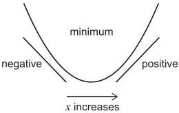
But why is this? The second derivative of a function can tell you how the first derivative is changing – usually whether the derivative is increasing or decreasing. If as $x$ increases the first derivative goes from negative to positive [see the diagram below] we have a minimum; and so, the derivative is usually increasing at a minimum (we are being cautious as the derivative at a minimum could also give $\frac{\mathrm{d}^2y}{\mathrm{d}x^2} = 0$ in some cases — see our discussion below). Hence, we know that if $\frac{\mathrm{d}^2y}{\mathrm{d}x^2} > 0$ at the stationary point – and recall the second derivative tells you how the first derivative is behaving – then there is a minimum.

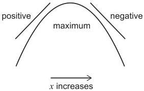
If as $x$ increases the derivative goes from positive to negative [see the diagram below] we have a maximum; and so, the derivative is usually decreasing at a maximum. Hence, we know that if $\frac{\mathrm{d}^2y}{\mathrm{d}x^2} < 0$ at the stationary point, then there is a maximum.

In the last bullet point above we were a little cautious in how we worded things. This is because we need to be careful about the logic of what we have said:

If (\frac{\mathrm{dy}}{\mathrm{dx}} = 0) and (\frac{\mathrm{d}^2y}{\mathrm{dx}^2} >0) then we have a minimum
If (\frac{\mathrm{dy}}{\mathrm{dx}} = 0) and (\frac{\mathrm{d}^2y}{\mathrm{dx}^2} < 0) then we have a maximum

And so:

the condition $\frac{dy}{dx} = 0$ and $\frac{d^2y}{dx^2} > 0$ is sufficient but not necessary for a minimum (see our Notes on Logic and Proof for a discussion of necessary and of sufficient).
the condition $\frac{dy}{dx} = 0$ and $\frac{d^2y}{dx^2} < 0$ is sufficient but not necessary for a maximum (see our Notes on Logic and Proof for a discussion of necessary and of sufficient).

Why is the condition only a sufficient condition and not a necessary one? The answer is that:

$\frac{dy}{dx} = 0$ and $\frac{d^2y}{dx^2} = 0$ could occur at a minimum [e.g. at $y = x^4$ ]
$\frac{dy}{dx} = 0$ and $\frac{d^2y}{dx^2} = 0$ could occur at a maximum [e.g. at $y = -x^4$ ]

In other words:

at a minimum we have $\frac{dy}{dx} = 0$ and we could have either $\frac{d^2y}{dx^2} > 0$ or $\frac{d^2y}{dx^2} = 0$ but not $\frac{d^2y}{dx^2} < 0$
at a maximum we have $\frac{dy}{dx} = 0$ and we could have either $\frac{d^2y}{dx^2} < 0$ or $\frac{d^2y}{dx^2} = 0$ but not $\frac{d^2y}{dx^2} > 0$

Strictly increasing and strictly decreasing functions

Now we can turn to look at strictly increasing and strictly decreasing functions in relation to differentiation (we have used a slightly narrow definition of strictly increasing and decreasing in the TMUA/ESAT as we wanted to relate the topic to differentiation without adding too many additional ideas to grasp; there are other definitions that take into account some of the subtle issues we discuss in this section – for instance, other definitions do not have to worry about functions with corners etc). We will not explore the other topics mentioned in MM6.3 as they are standard topics that we expect you to have fully covered in your mathematics course.

First, note that here the specification has been slightly changed when compared to previous TMUA specifications: strictly increasing and strictly decreasing has replaced increasing and decreasing.

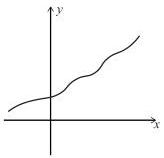
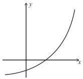
Let's start by developing an intuitive grasp for what a strictly increasing function is. In simple terms, a strictly increasing function is one that is always getting greater [the y value gets greater] as the x value gets greater. We could also say that it always slopes upwards. We have drawn some strictly increasing functions below.

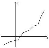
The same idea applies to strictly decreasing functions: they always get less [the y value gets less] as the x value gets greater. We could also say that it always slopes downwards. We have drawn some strictly decreasing functions below:

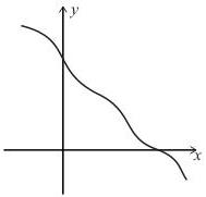
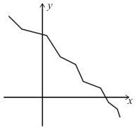
There are a few things to note in what we have said so far. First notice that we used the terms "greater" and "less" rather than "bigger" and "smaller". We did this because there can be some confusion if the y-values are negative: it might not be clear that -3 is "bigger" than -5, but it is true that -3 is greater than -5. Secondly, notice that some of the pictures in our examples deliberately have corners in them. We put these in to show that a function can increase but there might be place on the function where we cannot find the value of f'(x) – you cannot find the value for f'(x) on a corner as a corner does not have a unique tangent. Both these points are important for when we come to the definition and the logic we use in the TMUA/ESAT in relation to strictly increasing and strictly decreasing functions.

The way we have set out our definition does not capture all cases of strictly increasing/decreasing functions. You should pay careful attention to what the specification says:

if f'(x) > 0 then the function is strictly increasing
if f'(x) < 0 then the function is strictly decreasing

So, we have given a sufficiency condition for strictly increasing/decreasing but not a necessary one [there are necessary conditions that we could give but we are interested in the TMUA/ESAT at getting a feel for the shape of functions using differentiation so we have restricted what we have expected of you].

Notice that we CANNOT say:

If a function is strictly increasing, then f'(x) > 0 for all x
If a function is strictly decreasing, then f'(x) < 0 for all x

It should be clear we cannot say this – look at the examples we drew above and work our why these two statements are not true (think about what happens to $f'(x)$ when graphs have 'corners on them').

There is a little bit more we can say about strictly increasing and strictly decreasing functions: notice we have not yet said what $x$ values the conditions apply to. Usually we apply the definition to the whole domain of the function [the domain is all the $x$ values the function is defined on – usually this will be all real $x$ values, that is the whole $x$ -axis, unless otherwise stated, or unless the function is only defined on a subset of the real numbers, e.g. log functions]. We could look at restricted set of $x$ values in an obvious manner:

if $f'(x) > 0$ in $a < x < b$ then the function is strictly increasing in $a < x < b$
if $f'(x) < 0$ in $a < x < b$ then the function is strictly decreasing in $a < x < b$

A final note

In TMUA/ESAT, we will not test you on special cases and subtle technicalities for this topic. We do expect you to understand what is means for a nice graph [continuous – i.e. no breaks in the graph; with no sharp corners] to be strictly increasing or strictly decreasing and we will base our questions around simple functions such as polynomials which we know are well behaved. You won't need to worry about issues such as if the functions we use have corners and that sort of thing, but you do need to make sure you understand the logic of the definition we have decided to use.

Inflexions

For inflexions, we expect you to know what they are in general terms and where they might occur [e.g., in $y = x^3$ ] so that you can take account of their possibility when thinking about polynomials and their graphs. We do not expect you to have a detailed knowledge of how to identify a point of inflexion using differentiation and we will not ask questions that specifically involve technical issues directly related to points of inflexion.

Integration: introductory remarks

Before we start to look at the specification for this section, we have a few introductory remarks to make.

First, there are two ways to think about integration. These two ways are closely related but how they relate is not something we expect you to know for the TMUA/ESAT.

Either you can think of integration as the reverse of differentiation – it tells you what must have been differentiated to get the expression you are integrating.

Or, you can think of integration as finding the "area" between a curve and the $x$ -axis; but we have to be very careful by what we mean by "area" and that is something we shall discuss carefully below.

When integration is written as the reverse of differentiation it tends to look like this (sometimes [but not really until some university course on mathematics] integration can be written as $\int dx \, x^2$ ; this $\int$ is actually an elongated "s" meaning "sum" – it behaves similarly to $\Sigma$ ; the notation we use for calculus is largely derived from Leibnitz – look up "Leibnitz notation"):

$\int x^2 \, dx$

The expression being integrated appears between the $\int$ and the $dx$ and in this case the expression is asking "what must be differentiated to get $x^2$ ?" and the answer is

$\frac{x^3}{3} + c$

And note we add a constant term " $c$ " – you should be able to explain why we do this. [recall that when you differentiate a constant, you get 0]

When integration is asking you to find "areas" then we tend to have numbers written at the top and bottom of the $\int$ . In these cases, it is called "definite integration", and the numbers are called "limits". We will unpack some aspects of definite integration below. Here is an example of a definite integral:

$\int_1^3 x^2 \, dx$