Applications of Differentiation for the TMUA
Updated August 2025
This section covers the practical application of derivatives to analyse function behaviour. You will learn to determine gradients, tangents, and normals, as well as locate and classify stationary points using the second derivative. Mastering these techniques is vital for sketching polynomial curves and identifying where functions are strictly increasing or decreasing.
Stationary points occur where the gradient is zero, . These are classified as local maxima when and local minima when .
Gradients, Tangents, and Normals
Differentiation is used to find the rate of change of a curve at a specific point. This rate of change is defined as the gradient of the tangent to the curve at that point. By calculating , you obtain a function that gives the gradient for any value. The tangent at a point is a straight line with the same gradient as the curve at that point. The normal is the line perpendicular to the tangent at that point; its gradient satisfies the condition , where is the gradient of the tangent.
Identifying Stationary Points
Stationary points occur where the tangent to a curve is horizontal, meaning the gradient is zero. To find these points, you must solve the equation . These points are often referred to as local maxima or local minima because they represent the highest or lowest values of the function in a small local region, though they are not necessarily the global extremes of the function.
Worked Example
Consider the cubic . We can find the -coordinates of its stationary points by differentiating:
Setting this to zero to find the stationary points:
This gives stationary points at and .
Classifying Stationary Points
Once stationary points are located, they must be classified. There are three common techniques:
-
General Shape: For simple polynomials, the leading coefficient often dictates the shape. In the cubic example above, the positive coefficient implies the graph goes from bottom-left to top-right. Thus, the leftmost stationary point () must be a maximum and the rightmost () must be a minimum.
-
Neighbouring Values: You can check the values slightly to the left and right of the stationary point. If the values on both sides are larger than the value at the point, it is a minimum. If they are smaller, it is a maximum.
-
The Second Derivative Test: This is the most formal method. If at the stationary point, the gradient is increasing, indicating a minimum. If , the gradient is decreasing, indicating a maximum.
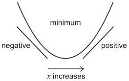
In the diagram above, the derivative goes from negative to positive, creating a minimum where the second derivative is positive.
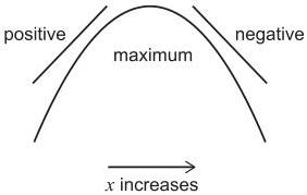
In this diagram, the derivative goes from positive to negative, creating a maximum where the second derivative is negative.
Logic of the Second Derivative Test
It is important to understand the logic of these conditions. The condition and is sufficient but not necessary for a minimum. This is because some minima, such as the origin on , have . Similarly, is a sufficient but not necessary condition for a maximum, as also has a zero second derivative at its maximum.
Strictly Increasing and Decreasing Functions
A strictly increasing function is one where the value always increases as increases. This is guaranteed if for all in a given interval. Conversely, a strictly decreasing function always slopes downwards, which is guaranteed if .
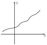
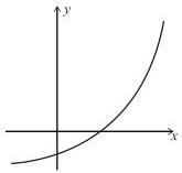
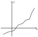
Note that these definitions using derivatives are sufficient conditions. We cannot say that if a function is strictly increasing, its derivative must be positive everywhere. For example, is strictly increasing over the whole real line, even though its gradient is zero at the origin. Also, functions with sharp corners can be strictly increasing without having a derivative at every point.
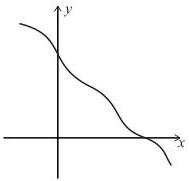
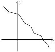
Qualitative Understanding of Points of Inflexion
Points of inflexion are where the curve changes from being 'convex' to 'concave' (or vice versa). While a technical analysis of inflexion points is not required, you should recognise them qualitatively. A classic example is at , where the stationary point is neither a maximum nor a minimum but a horizontal point of inflexion.
Key takeaways
- A stationary point is defined by the condition .
- A local minimum is confirmed if the second derivative at the stationary point.
- A local maximum is confirmed if the second derivative at the stationary point.
- A function is strictly increasing on an interval if for all in that interval.
- A zero second derivative at a stationary point is inconclusive; the point could be a maximum, a minimum, or an inflexion point.
When classifying stationary points of a polynomial, consider the coefficient of the highest power of . For a cubic with a positive coefficient, the first stationary point encountered from left to right is always the maximum and the second is the minimum.
Do not assume that automatically indicates a point of inflexion. As seen with , the second derivative can be zero at a local minimum.
The second derivative measures the rate of change of the gradient. If the gradient is zero and its rate of change is positive, the gradient must be moving from negative to positive, which geometrically creates a 'cup' shape or a local minimum.
Worked Examples
Practice Questions
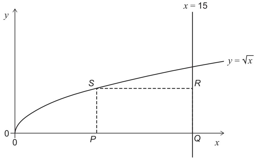
P and Q lie on the x-axis.
Q and R lie on the line
S lies on the curve
What is the maximum possible area of the rectangle?
Frequently asked questions
What happens if both the first and second derivatives are zero?
If and , the second derivative test is inconclusive. The point could be a maximum (like ), a minimum (like ), or a horizontal point of inflexion (like ).
Is a stationary point always a maximum or a minimum?
No, a stationary point can also be a horizontal point of inflexion, where the gradient is zero but the function does not change from increasing to decreasing or vice versa.
What is the difference between increasing and strictly increasing?
In the TMUA, a function is strictly increasing if . Strictly increasing means the value must actually get larger for every increase in , whereas 'increasing' sometimes allows for the function to stay flat (constant) for some intervals.